Database Indexing in MySQL Explained: B-Tree, Primary, Secondary, Composite Indexes and Selectivity

A beginner-friendly guide to database indexing in MySQL. Understand B-tree structure, primary, secondary and composite indexes, and how selectivity decides if an index helps.

Database indexing is one of those topics every backend developer runs into sooner or later. Maybe a query that used to be fast suddenly crawls. Maybe your boss asks why the reports page takes ten seconds to load. Most of the time, the answer comes back to indexes. In this guide, we will unpack database indexing in plain language, look at how the B-tree structure works under the hood, and understand primary, secondary, and composite indexes. We will also talk about selectivity, which is the idea that decides whether an index is even worth having.

I have kept the language simple and beginner friendly. You do not need a computer science degree to follow along. If you have written a few SQL queries and seen one run slowly, you already have enough background. Every example in this article uses MySQL, since that is what most Java shops run in production. Still, the core ideas carry over to PostgreSQL and other relational databases too.

Let us start with the basic question: what problem does an index actually solve?

1. What Is a Database Index?

Think about a thick textbook with a thousand pages. You want to find every mention of the word “transaction.” Without an index at the back of the book, you would flip through every single page. That is slow and painful. With an index, you jump to the letter T, find “transaction,” and it tells you the exact pages. You skip almost all the work.

A database index does the same job. It is a separate data structure. It stores a sorted copy of one or more columns, along with a pointer to the actual row. When you search on an indexed column, the database uses this structure to jump straight to the rows you want. It does not scan the whole table.

Here is the part that trips people up. An index is not the table itself. It is a helper stored alongside the table. It takes extra disk space, and it needs updating every time you insert, update, or delete a row. So indexes are not free. They speed up reads but slow down writes a little. The trick is knowing when the trade is worth it.

Before we go deeper, here is a quick map of the index types we will cover. Keep this list in mind as you read:

• Primary index: built on the primary key. In MySQL it is clustered, meaning it controls how rows are physically stored.
• Secondary index: any index that is not the primary key. It points back to the primary key to find the full row.
• Composite index: a single index built on two or more columns together.
• Covering index: a secondary index that already holds every column a query needs, so no extra lookup is required.
• Unique index: an index that also enforces that no two rows share the same value.

Do not worry if these terms feel fuzzy right now. We will unpack each one with examples. For now, just notice that they are all variations on the same B-tree idea.

1.1 Why Full Table Scans Hurt

When there is no useful index, the database does what we call a full table scan. It reads every row, checks each one against your condition, and keeps the matches. On a table with a few hundred rows, nobody notices. On a table with ten million rows, this becomes a real problem.

Say you run this query:

SELECT * FROM users WHERE email = 'ravi@example.com';

Without an index on email, MySQL reads all ten million rows to find maybe one match. With an index, it walks a small tree and lands on the row in a handful of steps. The difference is not small. It can turn a two second query into a two millisecond query.

A full table scan hurts in more than one way. It is worth spelling out where the pain comes from:

• CPU work: the database checks the condition against every single row, even the ones that clearly do not match.
• Disk reads: on a big table, most of the data does not fit in memory, so MySQL pulls pages from disk, which is slow.
• Cache pollution: scanning a huge table pushes useful data out of the buffer pool, which then slows down other queries too.
• Lock time: a long scan can hold locks longer, which makes other users wait.

An index attacks all of these at once. It reads far fewer pages, touches far fewer rows, and finishes fast enough that locks are released quickly.

2. The B-Tree: How Indexes Are Actually Stored

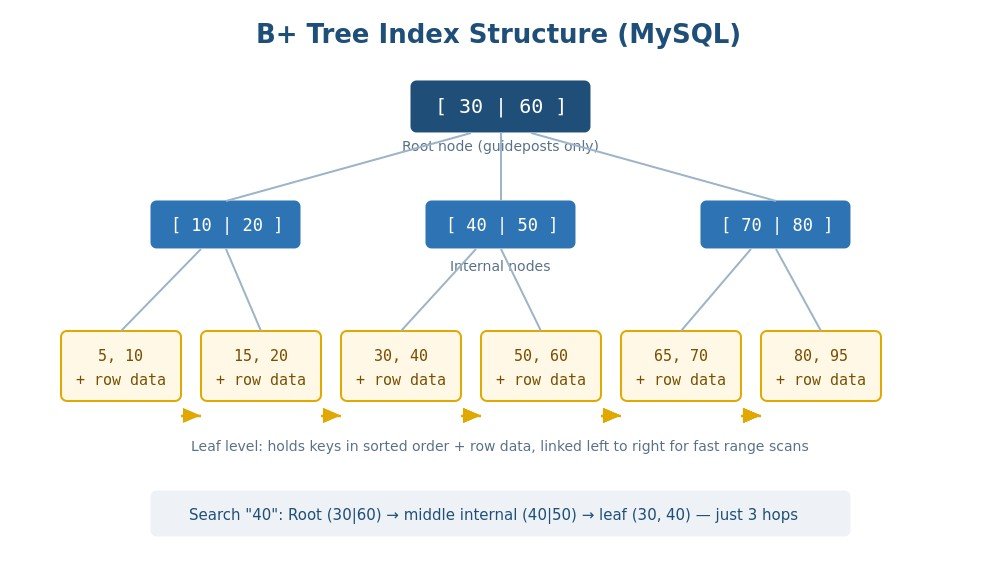
Most database indexes use a structure called a B-tree, or more precisely a B+ tree in the case of MySQL. The name sounds scary, but the idea is friendly once you picture it. Let us build the mental model step by step.

2.1 A Simple Picture of the Tree

Imagine a family tree turned upside down. At the very top sits one node, called the root. The root points down to a few child nodes. Each child points down to more nodes, and so on, until you reach the bottom layer, called the leaf level. The leaves hold the actual keys in sorted order.

When you search for a value, you start at the root. The root tells you which child to go to. That child narrows it down further. You keep moving down until you hit a leaf. Because each step throws away a big chunk of the data, you reach your target in very few hops.

Here is the key benefit. A B-tree stays balanced. Every leaf sits at the same depth. So whether you search for the first value or the last, the number of steps is roughly the same. For a table with a million rows, you might reach any row in three or four steps instead of a million.

2.2 Why B+ Trees for Databases

MySQL uses a B+ tree, which is a small twist on the plain B-tree. In a B+ tree, all the real data lives in the leaf nodes. The upper nodes only hold guideposts that tell you which way to go. On top of that, the leaf nodes are linked together like a chain.

That chain matters a lot. Say you ask for a range, like all users who signed up between January and March. The database finds the start of the range. Then it just walks along the linked leaves. No jumping back up the tree. This makes range queries and sorted reads very efficient.

So the short version is this. B+ trees give you fast single lookups, fast range scans, and they keep themselves balanced automatically. That combination is why almost every relational database leans on them.

2.3 Separator Values in the Upper Nodes

The upper nodes hold what we call separator values. These are not rows. They are signposts that split the data into ranges. Picture a root node like this:

                                                                                                                                                                                                    
                    [ 20 | 40 ]
                  /      |      \
           [5 | 10]  [26 | 30]  [45 | 50]

The 20 and 40 in the root are separator values. They tell the database which child to visit:

• If the search key is less than 20, go to the left child.
• If it is between 20 and 40, go to the middle child.
• If it is 40 or more, go to the right child.

One thing trips people up here. The values inside a leaf, like 5 and 10, are real keys from your table. But a label like “less than 20” is not a stored value. It is just a range that the separator implies. So separators guide the path, while leaves hold the actual data.

2.4 Walking Through a Real Search

Let us make this solid with a small employees table. Say the rows look like this:

employee_id | employee_name | department
------------|---------------|-----------
5           | Alice         | HR
10          | Bob           | HR
15          | Carol         | Finance
20          | David         | IT
26          | Eva           | IT
30          | Frank         | Sales
35          | Grace         | Sales
40          | Henry         | Finance
45          | Irene         | Marketing
50          | Jack          | Marketing

Now you add an index on employee_id:

CREATE INDEX idx_employee_id
    ON employees(employee_id);

MySQL may build a B-tree that looks roughly like this:

                    
                [  20    |      40 ]
                  /      |           \
    [5 | 10 | 15]  [20 | 26 | 30 | 35]  [40 | 45 | 50]

Suppose you run this query:

SELECT * FROM employees WHERE employee_id = 30;

Here is what happens, step by step:

1. Start at the root [20 | 40]. Compare 30 with the separators.

2. 30 is greater than 20 but less than 40, so go to the middle child.

3. In the middle leaf [20 | 26 | 30 | 35], find 30 and return the row: Frank, from Sales.

Notice how few steps that took. Two hops, and the database landed on the exact row. Without the index, it would have checked every row until it hit employee_id 30. On ten rows that is nothing, but on ten million rows it is the whole ballgame.

2.5 Can the Tree Get Deeper?

Yes. Our example had just a root and a leaf level, so depth was small. But real tables are bigger, and the tree grows to match. A larger index might look like this:

                         
                         [ 50 ]
                       /        \
                [20 | 35]        [70 | 85]
               /    |    \       /    |    \
          leaves...          leaves...

Now there is a middle layer, called internal nodes, sitting between the root and the leaves. Depth grows for a simple reason. When a node fills up, the database splits it into two. If the root itself fills up, the database makes a brand new root on top. That adds one level to the whole tree.

The good news is that depth grows very slowly. Because each node holds many keys, even a table with hundreds of millions of rows usually needs only a handful of levels. That is why B-tree lookups stay fast no matter how big the table gets.

2.6 Who Decides the Tree Shape?

A common beginner question is who controls all this structure. The answer is reassuring. The database engine handles the internals for you. You never hand-build a tree.

The engine automatically decides:

• The separator values in each node.
• When to split a node and when to add a level.
• The overall depth and balancing of the tree.
• How keys are laid out on disk pages.

You, the developer, decide the things that actually matter for design:

• Which columns to index.
• Whether an index is single-column or composite.
• The column order inside a composite index.
• Whether an index is unique, and when to create or drop indexes.

So your job is to make good choices about what to index. The engine takes care of the messy tree mechanics underneath.

2.7 What Happens During Writes

There is a cost to all this neatness. When you insert a new row, the database has to place the new key in the right spot in the tree. Sometimes a leaf node gets full and has to split into two. That split can ripple upward. It is usually cheap, but it is not zero. This is the write cost of indexes we mentioned earlier. Every index on a table adds a little overhead to each write.

3. Primary Index: The Backbone of the Table

Now that we understand the tree, let us look at the different kinds of indexes. The first one is the primary index, and in MySQL it is special.

3.1 The Clustered Index

In MySQL, the primary key is not just an index. It decides the physical order of the rows on disk. This is called a clustered index. The table itself is stored as a B+ tree, sorted by the primary key. The leaf nodes hold the full rows.

Let me say that again because it matters. In MySQL, the table and the primary key index are the same structure. The rows live inside the primary key’s B+ tree. There is no separate heap of rows sitting somewhere else.

Consider a simple table:

CREATE TABLE orders (
    id BIGINT PRIMARY KEY AUTO_INCREMENT,
    customer_id BIGINT,
    total DECIMAL(10,2),
    created_at DATETIME
);

Here, id is the clustered index. All order rows are physically arranged in order of id. When you look up an order by its id, MySQL walks the primary tree and finds the whole row at the leaf. One lookup, done.

3.2 Why Auto-Increment Keys Are Popular

Since MySQL stores rows in primary key order, the choice of primary key affects performance. An auto-increment integer is a friendly choice. New rows get bigger and bigger ids, so they always slot in at the end of the tree. No shuffling of existing data.

Compare that with a random primary key, like a UUID. New values land in random spots in the middle of the tree. This causes more page splits and more disk churn. Many teams still use UUIDs for good reasons, but it helps to know the cost. If you need UUIDs, look into ordered variants that keep inserts mostly sequential.

4. Secondary Index: Everything Else

A primary index is great, but you often search by other columns too. That is where secondary indexes come in. Any index that is not the primary key is a secondary index.

4.1 How a Secondary Lookup Works

A secondary index is also a B+ tree, but its leaves do not hold the full row. Instead, the leaves hold the indexed column value plus the primary key. So a secondary index points back to the primary key, not directly to the row.

This means a lookup by a secondary index can take two steps. First, the database searches the secondary tree and finds the primary key of the matching row. Second, it uses that primary key to walk the clustered index and fetch the full row. This second hop is often called a bookmark lookup.

Say you add an index on email:

CREATE INDEX idx_users_email ON users(email);

When you query by email, MySQL finds the email in the secondary tree, grabs the primary key stored there, then jumps to the clustered index to pull the rest of the columns. Two trees, two walks, still very fast compared to a full scan.

4.2 Covering Indexes: Skipping the Second Hop

Here is a neat trick. Sometimes the second hop is wasteful. If your query only needs the columns already sitting in the secondary index, the database can answer straight from the index. It never touches the clustered index at all. This is called a covering index.

Suppose you often run:

SELECT email FROM users WHERE email LIKE 'ravi%';

The idx_users_email index already holds email and the primary key. The query only asks for email. So MySQL answers from the index alone. No bookmark lookup. When you see “Using index” in an EXPLAIN output, that is a covering index doing its job.

5. Unique Indexes and Constraints

There is one more index type worth its own section, because it does double duty. A unique index is a normal B-tree index, but it also enforces a rule. It refuses to let two rows share the same value in the indexed column.

Say you want every user to have a distinct email. You can add a unique index:

CREATE UNIQUE INDEX idx_users_email_unique
    ON users(email);

Now if someone tries to insert a second row with an existing email, MySQL rejects it with a duplicate key error. So the index gives you two things at once:

• Speed: like any index, it makes lookups on email fast.
• Correctness: it guarantees no duplicate emails ever sneak into the table.

This is handy because you get data integrity for free. You were probably going to index email anyway. Making it unique adds a safety net at almost no extra cost.

A couple of small points are worth knowing. Note that a primary key is really a special unique index that also forbids NULL values. A plain unique index, on the other hand, usually allows one NULL, because in SQL two NULLs are not considered equal. So if a column can be empty, think about whether unique still makes sense for your case.

6. Composite Index: Indexing Multiple Columns

So far each index covered one column. But real queries often filter on several columns at once. A composite index, also called a multi-column index, covers two or more columns together in a single tree.

6.1 The Order of Columns Matters

This is the single most important rule about composite indexes, and it catches many developers. In a composite index, the order of columns is not just a detail. It changes what the index can do.

Picture an index on (customer_id, created_at). The database sorts first by customer_id, and then, within each customer, by created_at. It works like a phone book sorted by last name and then first name. You can find everyone with the last name “Sharma” easily. You can even find “Sharma, Anita.” But you cannot quickly find everyone named “Anita” across all last names. The first column drives everything.

6.2 The Leftmost Prefix Rule

Databases follow what is called the leftmost prefix rule. A composite index on (a, b, c) can help queries that filter on a, on a and b, or on a, b, and c. But it cannot help a query that filters only on b, or only on c.

Let us make it concrete. Given this index:

CREATE INDEX idx_orders_cust_date
    ON orders(customer_id, created_at);

These queries can use the index:

SELECT * FROM orders WHERE customer_id = 42;
 
SELECT * FROM orders
WHERE customer_id = 42 AND created_at > '2025-01-01';

But this next query cannot use the index efficiently, because it skips the leftmost column:

SELECT * FROM orders WHERE created_at > '2025-01-01';

Since customer_id is missing from the filter, the tree’s sort order is useless for this search. The database falls back to scanning. So when you design a composite index, put the column you always filter on first.

6.3 Picking the Right Column Order

A good rule of thumb is to lead with columns used in equality checks, then follow with columns used in ranges. Equality first, range later. An index on (status, created_at) works well for a query like “give me pending orders from last week.” Here status is an equality and created_at is a range. Flip the order and it works less well.

6.4 Comparing the Three Index Types

We have now met the three main index types. It helps to see them side by side, so you can pick the right one for a given query:

A quick way to remember it: primary is for one row by its key, secondary is for one other column, and composite is for a set of columns you always query together. Most real applications use a mix of all three.

7. Selectivity: The Deciding Factor

We have talked a lot about how indexes work. Now let us talk about when an index actually helps. This is where selectivity comes in. Honestly, it separates people who guess at indexes from people who reason about them.

7.1 What Selectivity Means

Selectivity measures how many distinct values a column has compared to the total number of rows. A column is highly selective when most of its values are unique. It is poorly selective when the same few values repeat over and over.

You can think of it as a simple ratio:

selectivity = number of distinct values / total number of rows

A value close to 1 means high selectivity. A value close to 0 means low selectivity.

7.2 High Selectivity vs Low Selectivity

Take an email column. Almost every user has a unique email, so its selectivity is very high, close to 1. An index on email is excellent. When you search one email, the index narrows a million rows down to one. That is a huge win.

Now take a gender column with values like “male,” “female,” and “other.” Its selectivity is very low. An index here narrows a million rows down to maybe three hundred thousand. The database often decides an index is slower here. Reading that many rows, with all those bookmark lookups, costs more than a plain scan. So it ignores the index.

The numbers make this stark. Say a table has one million rows and a gender column with just two values. The selectivity is 2 divided by 1,000,000, which is 0.000002. That is about as low as it gets. Now run a query for gender = ‘M’, and it might match 500,000 rows, half the table. To serve that with an index, the database would read half the index and then jump into the table half a million times. It is far cheaper to scan the table straight through. So the optimizer skips the index entirely.

This surprises people. You created an index, but the database refuses to use it. Nine times out of ten, the reason is low selectivity. The optimizer looked at the numbers and decided a scan was cheaper.

Most columns sit somewhere in the middle. Take a department column with four values: HR, IT, Sales, and Finance. On a small table its selectivity is only moderate. But on a big table, filtering by one department still trims the result to a quarter or less. So a department index can help on a large table, even though the same index would be pointless on a tiny one. Table size changes the answer.

Here is a quick way to picture the three cases:

• High selectivity, like email: almost every value is unique, so an index is a clear win.
• Medium selectivity, like department: an index may help on big tables and not on small ones.
• Low selectivity, like gender: each value matches so many rows that an index alone rarely pays off.

7.3 Why Too Many Matches Kill an Index

It helps to understand why a low selectivity index gets ignored. Using a secondary index is a two part job. First the database reads the index to find matching keys. Then it uses those keys to jump into the table and fetch each full row. That second jump is the expensive part.

When only a few rows match, those jumps are cheap and the index wins easily. But when half the table matches, the database faces hundreds of thousands of jumps to scattered locations. At that point, reading the whole table in order is often faster than hopping around. So the optimizer quietly drops the index and scans instead.

A book makes this click. Imagine you want one rare topic that appears on a single page. The book index is perfect: look it up, flip to that page, done. Now imagine the topic appears on half the pages. The index would list hundreds of page numbers, and chasing each one is slower than just reading the book straight through. An index on a low selectivity column is that second case.

7.4 Checking Selectivity Yourself

You do not have to guess. You can measure it with a quick query:

SELECT
    COUNT(DISTINCT status) AS distinct_values,
    COUNT(*) AS total_rows,
    COUNT(DISTINCT status) / COUNT(*) AS selectivity
FROM orders;

Run this on any column you are thinking of indexing. If the selectivity number is tiny, an index alone probably will not help much. You might still use that column inside a composite index. Pair it with a more selective column, and you get a good result.

7.5 Cardinality and the Optimizer

You will also hear the word cardinality. It is closely related. Cardinality is the count of distinct values in a column. High cardinality means high selectivity. The MySQL optimizer keeps cardinality statistics for each index. It uses them to decide whether an index is worth using for a given query. If those statistics go stale, the optimizer can make poor choices. Running ANALYZE TABLE refreshes them.

8. When to Add an Index, and When to Skip It

An index is a tool, not a reflex. Before we list the traps, it helps to know when an index genuinely earns its place. Reach for one in these cases:

• The query returns only a few rows out of many. This is the classic win.
• The filter column has high selectivity, like an email or a user id.
• You filter on the column often in your WHERE clauses.
• You join two tables on the column. An index on the join key speeds the join a lot.
• You sort by the column with ORDER BY. A matching index can skip a separate sort step.
• A composite index lines up with a query that filters several columns together.

Now the other side. New developers often think more indexes are always better. That is not true. Each index you add makes writes a little slower and takes disk space. On a busy table, this adds up. So it helps to know when an index is a bad idea.

Think twice before indexing in these situations:

• Small tables. If a table has only a few hundred rows, a full scan is already fast. An index barely helps and just adds overhead.
• Write-heavy tables. If a table gets thousands of inserts per second, every extra index slows those writes. Keep indexes lean here.
• Low selectivity columns. As we will see, a column with only a handful of distinct values rarely benefits from a standalone index.
• Columns you never filter or sort on. An index on a column no query touches is pure waste. It costs writes and gives nothing back.
• Wide columns. Indexing a long text column makes a big, slow index. If you must, index a prefix of the column instead of the whole thing.

A simple habit keeps you honest. Before adding an index, ask: which real query will this speed up? If you cannot name one, do not add it. Indexes should follow your query patterns, not your fears.

It also pays to review indexes now and then. Applications change. A query that ran a hundred times a day last year might be gone now, leaving a dead index behind. MySQL can even tell you which indexes go unused, so you can drop the ones that only cost you writes.

9. A Light Java Example

Since many readers come from a Java and Spring background, let us tie this back to code briefly. The database does the heavy lifting, but the way you write queries in JPA affects which indexes get used.

Suppose you have a Spring Data repository:

public interface OrderRepository
        extends JpaRepository<Order, Long> {
 
    List<Order> findByCustomerIdAndCreatedAtAfter(
            Long customerId, LocalDateTime after);
}

This method generates SQL that filters on customer_id and created_at, in that order. It maps neatly onto our composite index idx_orders_cust_date. The leftmost column, customer_id, comes first in the filter, so the index gets used.

Now compare a method that only filters on the second column:

List<Order> findByCreatedAtAfter(LocalDateTime after);

This one filters on created_at alone. It cannot use the composite index efficiently, because created_at is not the leftmost column. If this query runs often on a big table, you would want a separate index that leads with created_at. The lesson is simple. Your Java method names quietly decide your SQL, and your SQL decides your index usage.

10. Common Indexing Mistakes to Avoid

Let us close the main content with a short list of traps I see again and again. These are easy to fix once you know them.

1. Indexing every column just in case. Each index slows writes and eats disk. Add indexes for real query patterns, not for imagined ones.

2. Ignoring column order in composite indexes. Remember the leftmost prefix rule. The wrong order makes the index useless for your query.

3. Indexing low selectivity columns on their own. A standalone index on a status flag or a boolean rarely helps.

4. Forgetting that functions block indexes. A query like WHERE YEAR(created_at) = 2025 cannot use a plain index on created_at, because the function hides the raw value. Rewrite it as a range instead.

5. Never checking EXPLAIN. The EXPLAIN keyword shows you exactly how MySQL plans to run a query and whether it uses your index. Make it a habit.

11. How to Verify Your Indexes Are Working

The best way to trust an index is to check it, not assume it. Put EXPLAIN in front of any query and read the output:

EXPLAIN SELECT * FROM orders
WHERE customer_id = 42
AND created_at > '2025-01-01';

Look at the type column. A value of “ref” or “range” usually means an index is being used well. A value of “ALL” means a full table scan, which is a warning sign on a big table. Look at the key column too, since it names the index actually chosen. If it shows NULL, no index was used. These two columns alone tell you most of what you need.

When you read an EXPLAIN output, these are the columns worth focusing on first:

• type: how MySQL finds rows. “const” and “ref” are great, “range” is fine, “index” scans the whole index, and “ALL” scans the whole table.
• key: the index MySQL actually chose. A NULL here means no index was used at all.
• rows: the estimated number of rows MySQL will examine. Lower is better.
• Extra: watch for “Using index” (a covering index, very good) and “Using filesort” or “Using temporary” (often a sign your index does not cover the sort).

The rows column is also worth a glance. It shows roughly how many rows MySQL expects to read. A small number is good. A number close to your table size means the query is doing far more work than it should. On newer MySQL versions, you can add the FORMAT=JSON option or use EXPLAIN ANALYZE to see real timings, not just estimates. That extra detail helps when two plans look similar on paper.

One more habit worth building is testing on realistic data. An index that looks pointless on a hundred rows can become essential on a million. So try to run EXPLAIN against a copy of production-sized data, not a tiny local table. The optimizer changes its mind based on table size, and you want to see the decision it will actually make in production.

12. Interview Questions

13. Conclusion

Indexes are not magic, but they can feel like it when a slow query suddenly flies. The core ideas are steady. A B-tree, or B+ tree in MySQL, keeps your data sorted and balanced so lookups take just a few steps. The primary index is clustered and holds your rows in key order. Secondary indexes point back to the primary key and sometimes cover a query on their own. Composite indexes combine columns, but only help when you respect the leftmost prefix rule. And selectivity decides whether any index is worth the space at all.

Get comfortable with EXPLAIN, measure selectivity before you add an index, and think about the real queries your application runs. Do that, and you will spend far less time staring at slow query logs. Indexing stops being guesswork and becomes something you can reason about with confidence.

If you remember nothing else, hold on to these five points:

• A B+ tree keeps data sorted and balanced, so lookups take only a few steps even on huge tables.
• In MySQL, the primary key is a clustered index and decides how rows sit on disk.
• Secondary indexes point back to the primary key, and a covering index can skip that second hop.
• Composite indexes only help when your filter respects the leftmost prefix rule.
• Selectivity decides whether an index is worth it. High selectivity helps, low selectivity often does not.

Further Reading

• MySQL official documentation on how MySQL uses B-tree indexes and the clustered index layout.
• MySQL EXPLAIN output reference, for reading query execution plans in detail.
• PostgreSQL indexing documentation, useful for comparing how another database handles the same ideas.