Stream Processing with Kafka Streams: Windowing and Backpressure Explained

Stream processing with Kafka Streams made simple. Learn tumbling, hopping, sliding & session windows, plus how to handle backpressure and consumer lag.

Most systems we build early in our careers work in batches. Data lands in a table, a job wakes up at midnight, it crunches the numbers, and a report shows up in your inbox. That worked fine for years. But users now expect things to happen right away. They want the fraud alert before the payment clears, not the next morning. This is exactly where stream processing with Kafka Streams comes in, and it changes how you think about data from the ground up.

In this article we will walk through what stream processing actually means, how Kafka Streams handles it, and two topics that trip up almost everyone at first: windowing and backpressure. I have kept the language simple on purpose. If you have used Kafka even a little, you will follow along fine. And if you are prepping for a system design interview, I have added short interview notes along the way so you can spot what matters.

1. What Stream Processing Really Means

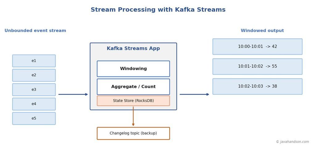
Let us start with a plain picture. A batch job treats data as a big bucket that sits still. You wait for the bucket to fill, then you process the whole thing at once. Stream processing treats data as water flowing through a pipe. There is no end to the pipe. Events keep coming, one after another, and you process each one as it passes by.

That single shift has big effects. Because the stream never ends, you can never say “process everything and stop.” Instead, you process forever. So your code has to be ready for data at any moment, and it has to keep going even when traffic spikes or slows down.

Here are the traits that make a stream different from a batch:

• It is unbounded. New events can always arrive, so there is no final record.
• It is ordered within a partition. Events carry timestamps, and order matters a lot.
• It is continuous. Your program runs all day and all night, not for a fixed run.
• It is often stateful. To answer real questions, you must remember what you saw earlier.

That last point matters more than people expect. Counting clicks per user, for example, means you must hold a running total somewhere. So state is not a side detail. It sits right at the heart of stream processing.

2. Where Kafka Streams Fits

Apache Kafka, on its own, is a log. Producers write events to topics, and consumers read them back. That is powerful, but it is fairly low level. If you want to group events, count them, or join two streams together, you end up writing a lot of plumbing by hand. You track offsets, you manage threads, you store partial results, and you handle failures. It gets messy fast.

Kafka Streams is a library that sits on top of that log and does the heavy lifting for you. It is not a separate cluster you have to run. It is just a Java library you add to your app. Your service starts up, connects to Kafka, and starts processing. So there is no extra system to babysit, which teams really appreciate.

Because it is only a library, you deploy it like any normal application. You can run one instance or ten. When you add more instances, Kafka Streams spreads the work across them automatically. It does this using the same consumer group mechanism that plain Kafka consumers use. So scaling out is mostly a matter of starting more copies.

A few things Kafka Streams gives you for free:

• Automatic offset handling, so you do not track read positions by hand.
• Built-in state stores, backed by local RocksDB and restored from Kafka on restart.
• Exactly-once processing, when you turn it on, so records are not double counted.
• Windowing and joins as first-class operations, not something you build yourself.

This is the reason so many teams reach for it. You get the correctness guarantees of Kafka without writing them yourself. And you keep your simple deployment model, which is a rare combination.

One more thing worth clearing up early. People sometimes mix up Kafka Streams with heavier engines like Flink or Spark Streaming. Those are full frameworks that run on their own clusters, which you set up and manage. Stream processing with Kafka Streams stays lighter on purpose. It runs inside your service, so it fits teams who want power without a new cluster to operate. So the choice often comes down to how much operational weight you want to carry.

3. Core Building Blocks: KStream, KTable, and State

Before we get to windows, you need two ideas: the KStream and the KTable. They look similar in code, but they mean very different things. Getting them mixed up is one of the most common beginner errors, so let us slow down here.

3.1 KStream: a record of events

A KStream is a stream of facts that happened. Each record stands on its own. Think of a log of page views. If the same user views three pages, you get three separate events, and all three count. Nothing overwrites anything. It is append-only, just like a diary.

So when you read a topic as a KStream, you are saying “treat every record as a new independent event.” This fits things like clicks, payments, sensor readings, and orders.

3.2 KTable: the latest value per key

A KTable is different. It holds the latest value for each key, like a row in a database that keeps getting updated. If a user changes their email three times, you do not keep three emails. You keep the last one. Older values are replaced.

So a KTable is a changelog view. Same key, new value, and the old value is gone. This fits things like account balances, current status, and configuration that changes over time.

// Read a topic as a stream of events (append-only)
KStream<String, Order> orders =
    builder.stream("orders-topic");
 
// Read a topic as a table of latest values per key
KTable<String, Customer> customers =
    builder.table("customers-topic");
 
// Enrich each order with the customer's current details
KStream<String, EnrichedOrder> enriched =
    orders.join(customers,
        (order, customer) -> new EnrichedOrder(order, customer));

Notice the join above. An order event picks up the customer’s current details as it flows through. That is a stream-table join, and it is one of the most useful patterns you will use. The stream drives the action, and the table provides context.

4. Windowing: Slicing an Endless Stream into Chunks

Now we hit the topic that confuses most people. A stream never ends. So how do you answer a question like “how many orders came in this minute?” You cannot wait for the stream to finish, because it never will. This is the exact problem that windowing solves.

A window is a slice of time. Instead of counting forever, you count within a bucket. “Orders in the 10:00 to 10:01 bucket,” then “orders in the 10:01 to 10:02 bucket,” and so on. Each window gives you a finite group you can actually aggregate.

Kafka Streams gives you four window types. They sound similar, but each answers a slightly different question. Let us go through them one by one, because picking the wrong one leads to wrong numbers.

4.1 Tumbling Windows

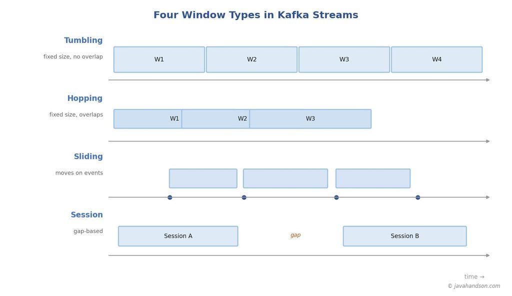
A tumbling window is the simplest one. It has a fixed size, and the windows never overlap. Picture a row of boxes lined up back to back. Every event falls into exactly one box. When one box ends, the next one begins right away.

So if you use a one-minute tumbling window, you get a clean count for 10:00 to 10:01, then a fresh count for 10:01 to 10:02. No event is counted twice. This is the window you want for things like “requests per minute” or “sales per hour.”

// Count orders in fixed, non-overlapping one-minute buckets
KTable<Windowed<String>, Long> orderCounts = orders
    .groupByKey()
    .windowedBy(
        TimeWindows.ofSizeWithNoGrace(Duration.ofMinutes(1)))
    .count();

4.2 Hopping Windows

A hopping window also has a fixed size, but it advances by a smaller step. So the windows overlap. Imagine a five-minute window that hops forward every one minute. An event near a boundary can land in more than one window at the same time.

Why would you want overlap? Smoothing. A five-minute view that updates every minute gives you a moving trend without waiting a full five minutes for each update. So it is great for dashboards and rolling averages. Just remember that overlapping windows mean an event gets counted in several windows, which is by design here.

// Five-minute window that advances every one minute (overlaps)
KTable<Windowed<String>, Long> rolling = orders
    .groupByKey()
    .windowedBy(TimeWindows
        .ofSizeWithNoGrace(Duration.ofMinutes(5))
        .advanceBy(Duration.ofMinutes(1)))
    .count();

4.3 Sliding Windows

A sliding window looks like a hopping window at first, but the trigger is different. It does not move on a fixed clock step. Instead, it moves based on the events themselves. A new window boundary appears whenever a record enters or leaves the time range.

In practice, this gives you a result for every distinct combination of events inside the window size. So it is more precise for things like “how many events happened within any 30-second span.” It costs more to compute, but the numbers are tighter. Use it when exact co-occurrence matters.

4.4 Session Windows

Session windows are the odd one out, and honestly the most interesting. They are not driven by the clock at all. They are driven by activity. A session stays open as long as events keep arriving close together. When there is a quiet gap longer than a limit you set, the session closes.

This maps perfectly to real user behavior. Someone browses a shop, clicks around for a few minutes, then leaves. That burst of activity is one session. If they come back an hour later, that is a new session. You set the inactivity gap, and Kafka Streams draws the boundaries for you based on the data.

// A session closes after 5 minutes of inactivity per key
KTable<Windowed<String>, Long> sessions = clicks
    .groupByKey()
    .windowedBy(
        SessionWindows.ofInactivityGapWithNoGrace(
            Duration.ofMinutes(5)))
    .count();

4.5 Late Events and the Grace Period

Here is a hard truth about the real world: events arrive late. A phone loses signal, a network hiccups, and an event that happened at 10:00 shows up at 10:03. So the question becomes, do you still count it in the 10:00 window, or do you drop it?

The grace period answers that. It is a small extra wait you allow after a window ends. During the grace period, late events for that window are still accepted. Once the grace period passes, the window is closed for good, and later events are dropped.

So you are trading speed against completeness. A short grace period gives fast results but may miss stragglers. A long one catches more late data but delays your final answer. There is no perfect setting. You pick based on how late your data usually is and how fast you need results.

One practical tip from experience: measure your real lateness before guessing. Look at the gap between event time and arrival time in production. Most teams are surprised by how long the tail actually is, and they set the grace period too short at first.

5. Stateful Processing and State Stores

Every window we just discussed needs memory. To count orders in a minute, the app must hold that running count somewhere until the window closes. That memory is called a state store, and it is worth understanding how it works, because it affects both correctness and recovery.

Kafka Streams keeps state locally on each instance, usually in RocksDB, which is a fast embedded key-value store. So reads and writes are quick because they are on local disk, not over the network. That local speed is a big part of why Kafka Streams performs well.

But local state raises an obvious worry. What happens if the instance crashes? You would lose the counts. Kafka Streams solves this cleanly. Every change to a state store is also written to a special Kafka topic called a changelog. So the state is backed up in Kafka itself.

When an instance restarts, or when work moves to another instance, the state store rebuilds from that changelog. So no data is lost, and the counts continue where they left off. This is the quiet magic that makes stateful streaming safe to run in production.

• Local first: state lives on the instance for speed, backed by RocksDB.
• Backed up always: every update is mirrored to a changelog topic in Kafka.
• Restored automatically: on restart or rebalance, the store rebuilds from the changelog.
• Sized carefully: large state means longer restore times, so watch your key space.

6. Backpressure: When Consumers Can’t Keep Up

Let us move to the second topic that catches people off guard. Backpressure is what happens when data arrives faster than your app can process it. The upstream is fast, the downstream is slow, and the gap keeps growing. If you ignore it, memory fills up, latency climbs, and eventually something falls over.

You see this all the time. A marketing campaign doubles traffic overnight. Then a downstream database gets slow. Later, a single heavy record jams the pipeline. Suddenly your consumers are behind, and the lag chart is climbing. So knowing how to handle this is a core skill, not an edge case.

6.1 Why Kafka’s Pull Model Helps

Here is some good news. Kafka is built in a way that handles backpressure more gracefully than many other systems. The reason is the pull model. In a push system, the source shoves data at you whether you are ready or not. That is how consumers get overwhelmed and crash.

Kafka works the other way. Consumers pull data when they are ready. If your app is busy, it simply asks for the next batch a little later. Meanwhile, the data waits safely in the Kafka topic. So the topic itself acts as a giant buffer that absorbs the spike.

This is a big deal. Because Kafka stores data on disk and keeps it for a set retention time, a slow consumer does not lose anything. It just falls behind for a while and catches up later. So the failure mode is delay, not data loss, which is far easier to live with.

6.2 The Knobs That Matter

Even with the pull model, you still need to tune things. A few consumer settings shape how backpressure behaves, and knowing them helps you react fast when lag appears.

• max.poll.records controls how many records you fetch in one poll. Lower it if each record is heavy, so you do not bite off more than you can chew.
• max.poll.interval.ms is how long Kafka waits before it decides your consumer is stuck. If processing takes too long, Kafka kicks the consumer out and rebalances.
• The pause and resume API lets you stop fetching from a partition when a buffer fills, then start again when there is room. This is manual backpressure control.
• Consumer group size decides how work is spread. More instances means more parallel processing, up to the number of partitions.

That last point has a hard limit worth remembering. You cannot have more active consumers than partitions in a group. If a topic has six partitions, a seventh consumer just sits idle. So partition count sets the ceiling on how far you can scale out.

// Tune the consumer to take smaller, safer bites
props.put(ConsumerConfig.MAX_POLL_RECORDS_CONFIG, 100);
props.put(ConsumerConfig.MAX_POLL_INTERVAL_MS_CONFIG, 300000);
 
// Manually apply backpressure when a downstream buffer is full
if (buffer.isFull()) {
    consumer.pause(consumer.assignment());
} else {
    consumer.resume(consumer.assignment());
}

6.3 Strategies When Lag Grows

So the lag chart is climbing. What do you actually do? There is no single fix, but there is a clear playbook. Start by finding the real cause, then apply the right lever. Here are the moves that work most often.

• Scale out consumers. Add more instances, up to the partition count, to process in parallel.
• Add partitions. If you are already at the partition ceiling, more partitions unlock more parallelism.
• Speed up processing. Often the fix is downstream, like a slow database call or a missing index.
• Batch smartly. Group work, such as bulk database writes, so each record costs less.
• Shed load. During extreme spikes, sample or drop non-critical events to protect the core path.

One warning from the field. Adding partitions later is not free. It changes how keys map to partitions, which can break the ordering you relied on. So plan partition counts early, and give yourself headroom. Changing them under pressure is stressful and risky.

7. A Beginner Walkthrough: Counting Orders per Minute

Let us tie it all together with a small example you could actually run. Say you run a shop, and you want a live count of orders per minute. It sounds simple, but it touches streams, windows, and state all at once. So it is a perfect first project.

Here is the plan in plain words. First, read the orders topic as a KStream. Next, group the orders so they can be counted together. Then, apply a one-minute tumbling window. Finally, count the orders in each window and write the result out. That is the whole flow.

StreamsBuilder builder = new StreamsBuilder();
 
// 1. Read orders as an append-only stream of events
KStream<String, Order> orders =
    builder.stream("orders-topic");
 
// 2. Group and window into clean one-minute buckets
KTable<Windowed<String>, Long> perMinute = orders
    .groupBy((key, order) -> order.getStoreId())
    .windowedBy(
        TimeWindows.ofSizeAndGrace(
            Duration.ofMinutes(1),
            Duration.ofSeconds(10)))
    .count();
 
// 3. Send the counts to an output topic
perMinute.toStream()
    .map((windowedKey, count) -> KeyValue.pair(
        windowedKey.key(),
        count))
    .to("orders-per-minute");
 
KafkaStreams streams =
    new KafkaStreams(builder.build(), props);
streams.start();

Let us read the code slowly. The groupBy line decides what we count by, which is the store id here. Next, windowedBy sets a one-minute tumbling window with a ten-second grace period, so slightly late orders still count. Finally, the count call does the actual math and keeps the running total in a state store.

Now think about what happens under the hood. As orders flow in, each one lands in the right minute bucket. The count in that bucket goes up. When the minute ends and the grace period passes, the window closes, and the final count is emitted. Meanwhile, the state store is quietly backed up to a changelog topic, so a crash cannot lose your counts.

That is the beauty of it. You wrote maybe twenty lines. But you got windowing, state, fault tolerance, and scaling for free. If you start a second instance of this app, Kafka Streams splits the partitions between them, and your throughput roughly doubles. So a tiny amount of code buys you a lot of power.

8. Common Mistakes and How to Avoid Them

I will close with the traps I see most often. These are the things that look fine in a demo but cause pain in production. Knowing them ahead of time saves you a lot of late-night debugging.

8.1 Confusing event time with processing time

Windows can use the time an event happened, or the time your app processed it. These are not the same, especially with late data. If you count by processing time, a delayed batch of events all lands in the wrong window. So decide early which time you mean, and be explicit about it.

8.2 Setting the grace period too short

New teams often set no grace period at all, or a tiny one. Then they wonder why their counts look low during network blips. Late events get dropped silently. So measure real lateness first, then set a grace period that matches it. Do not just guess.

8.3 Ignoring state store size

Session windows and long windows can hold a lot of state. If your key space is huge, the state store grows, and restarts get slow because the changelog must replay. So keep an eye on state size, and clean up old windows you no longer need.

8.4 Treating backpressure as a crash, not a signal

Rising lag is not a failure. It is a signal that says your app needs help. So set up alerts on consumer lag early. Then, when lag climbs, you have time to scale out or fix the bottleneck before users notice anything. The teams that monitor lag sleep better.

Get these four right, and you are ahead of most people who pick up Kafka Streams. The library handles the hard parts, but these choices are still yours to make. So make them on purpose, not by accident.

Let me leave you with the big picture. Stream processing feels strange at first because there is no end to the data. But once the window idea clicks, the rest follows. You slice time into buckets, you keep a little state, and you watch your lag. So start small, run the order-counting example, and build up from there. That hands-on habit is how the ideas really stick.

9. FAQ’s on stream processing with Kafka Streams

10. Conclusion

Stream processing feels odd at first because the data never stops. But once a few ideas click, the rest falls into place. You slice an endless stream into windows, you keep a little state, and you let Kafka’s pull model soak up the spikes. That is really the whole game.

Kafka Streams is a good place to start because it hides the hard parts. You get windowing, state stores, fault tolerance, and scaling without running a separate cluster. So you can focus on the question you actually want to answer, not the plumbing.

Keep the two big lessons close. Pick the right window for the question, whether that is tumbling, hopping, sliding, or session. And treat rising consumer lag as a signal, not a crash, so you can react before users notice. Get those right, and stream processing with Kafka Streams stops feeling scary and starts feeling like a tool you reach for often.

Further Reading

If this article helped, these related pieces on the blog go deeper into the surrounding topics:

• Apache Kafka Deep Dive: partitions, consumer groups, offsets, and ordering guarantees.
• Consistency Models Explained: strong, eventual, causal, and read-your-writes.
• Database Replication: how data stays in sync across nodes.
• Sharding and Partitioning Strategies: splitting data for scale.
• Kafka deep dive